Relative Frequency Distributions and Histograms

Contributed by:

NEO Fri, Feb 04, 2022 11:15 AM UTC

This pdf includes the following topics:-
Frequency histograms
Relative frequency distributions
Relative frequency histograms
Common distribution shapes

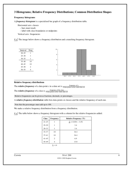
1. 3 Histograms; Relative Frequency Distributions; Common Distribution Shapes
Frequency histograms
A frequency histogram is a specialized bar graph of a frequency distribution table.
Horizontal axis: classes
– bars must touch
– label with class boundaries or midpoints
Vertical axis: frequencies
E.g. The image below shows a frequency distribution and a matching frequency histogram.
Interval Freq
20–25 1
25–30 1
30–35 1
35–40 10
40–45 10
45–50 2
50–55 4
Relative frequency distributions
frequency of x
The relative frequency of a data point x in a data set is # data points in the whole data set
frequency of the class
The relative frequency of a class is # data points in the whole data set
Relative frequencies can be given as fractions, decimals, or percentages.
A relative frequency distribution table lists data points or classes and the relative frequency of each one.
Note that the percentages must add up to 100.
We make a relative frequency distribution from a frequency distribution.
E.g. The table below shows a frequency histogram with a column for the relative frequencies added.
Class Frequency Relative Frequency (%)
1
21–25 1 29 ≈ 0.034 = 3.4%
25–29 1 3.4
29–33 1 3.4
33–37 10 34.4
37–41 10 34.4
41–45 2 6.9
45–49 4 13.8
∑ f =29
Corwin S TAT 200 6
©2011-2020 Stephen Corwin

2. Relative frequency histograms
A relative frequency histogram is a histogram for a relative frequency distribution.
E.g. The relative frequency histogram shown below matches the frequency distribution shown.
Class Frequency Relative
Frequency (%)
20–25 1 3.4
25–30 1 3.4
30–35 1 3.4
35–40 10 34.5
40–45 10 34.5
45–50 2 6.9
50–55 4 14.0
Σ f = 29
The Greek capital letter sigma (Σ) means “add up the values” (i.e., “sum”). Notice that the sum of the frequencies is the
total number of data points.
Corwin S TAT 200 7
©2011-2020 Stephen Corwin

3. E.g. Consider the following data set.
44 39 42 37 39 40 37 36 38 43
41 43 37 36 41 39 40 38 40 43
(a) Construct a frequency distribution for the data set using the classes 34–37, 37–40, 40–43, 43–46.
Class Frequency
34–37 2
37–40 8
40–43 6
43–46 4
(b) Construct a frequency histogram for the data set.
(c) Add a relative frequency column to your frequency distribution table.
Class Frequency Rel Freq (%)
2
34–37 2 20 = 0.1
37–40 8 0.4
40–43 6 0.3
43–46 4 0.2
(d) Construct a relative frequency histogram for the data set.
Corwin S TAT 200 8
©2011-2020 Stephen Corwin

4. Common distribution shapes
Note that (i) distributions don’t have to be exact and (ii) lots of distributions are symmetrical, but only the one that is symmet-
rical and has a single central hump is called the symmetric distribution.
Corwin S TAT 200 9
©2011-2020 Stephen Corwin

Book a Trial Class

download Download